Showing posts with label SQL. Show all posts

Graph RAG vs SQL RAG

Mike's Notes

Great explanation. Pipi uses both.

Resources

References

  • Reference

Repository

  • Home > Ajabbi Research > Library > Subscription > Towards Data Science
  • Home > Handbook > 

Last Updated

09/11/2025

Graph RAG vs SQL RAG

By: Reinhard Sellmair
Towards Data Science: 01/11/2025

.


Image generated with ChatGPT

I stored a Formula 1 results dataset in both a graph database and a SQL database, then used various large language models (LLMs) to answer questions about the data through a retrieval-augmented generation (RAG) approach. By using the same dataset and questions across both systems, I evaluated which database paradigm delivers more accurate and insightful results.

Retrieval-Augmented Generation (RAG) is an AI framework that enhances large language models (LLMs) by letting them retrieve relevant external information before generating an answer. Instead of relying solely on what the model was trained on, RAG dynamically queries a knowledge source (in this article a SQL or graph database) and integrates those results into its response. An introduction to RAG can be found here.

SQL databases organize data into tables made up of rows and columns. Each row represents a record, and each column represents an attribute. Relationships between tables are defined using keys and joins, and all data follows a fixed schema. SQL databases are ideal for structured, transactional data where consistency and precision are important — for example, finance, inventory, or patient records.

Graph databases store data as nodes (entities) and edges (relationships) with optional properties attached to both. Instead of joining tables, they directly represent relationships, allowing for fast traversal across connected data. Graph databases are ideal for modelling networks and relationships — such as social graphs, knowledge graphs, or molecular interaction maps — where connections are as important as the entities themselves.

Data

The dataset I used to compare the performance of RAGs contains Formula 1 results from 1950 to 2024. It includes detailed results at races of drivers and constructors (teams) covering qualifying, sprint race, main race, and even lap times and pit stop times. The standings of the drivers and constructors’ championships after every race are also included.

SQL Schema

This dataset is already structured in tables with keys so that a SQL database can be easily set up. The database’s schema is shown below:

SQL Database Design

Races is the central table which is linked with all types of results as well as additional information like season and circuits. The results tables are also linked with Drivers and Constructors tables to record their result at each race. The championship standings after each race are stored in the Driver_standings and Constructor_standings tables.

Graph Schema

The schema of the graph database is shown below:

Graph Database Design

As graph databases can store information in nodes and relationships it only requires six nodes compared to 14 tables of the SQL database. The Car node is an intermediate node that is used to model that a driver drove a car of a constructor at a particular race. Since driver – constructor pairings are changing over time, this relationship needs to be defined for each race. The race results are stored in the relationships e.g. :RACED between Car and Race. While the :STOOD_AFTER relationships contain the driver and constructor championship standings after each race.

Querying the Database

I used LangChain to build a RAG chain for both database types that generates a query based on a user question, runs the query, and converts the query result to an answer to the user. The code can be found in this repo. I defined a generic system prompt that could be used to generate queries of any SQL or graph database. The only data specific information was included by inserting the auto-generated database schema into the prompt. The system prompts can be found here.

Here is an example how to initialize the model chain and ask the question: “What driver won the 92 Grand Prix in Belgium?”

from langchain_community.utilities import SQLDatabase
from langchain_openai import ChatOpenAI
from qa_chain import GraphQAChain
from config import DATABASE_PATH

# connect to database
connection_string = f"sqlite:///{DATABASE_PATH}"
db = SQLDatabase.from_uri(connection_string)

# initialize LLM
llm = ChatOpenAI(temperature=0, model="gpt-5")

# initialize qa chain
chain = GraphQAChain(llm, db, db_type='SQL', verbose=True)

# ask a question
chain.invoke("What driver won the 92 Grand Prix in Belgium?")

Which returns:

{'write_query': {'query': "SELECT d.forename, d.surname
FROM results r
JOIN races ra ON ra.raceId = r.raceId
JOIN drivers d ON d.driverId = r.driverId
WHERE ra.year = 1992
AND ra.name = 'Belgian Grand Prix'
AND r.positionOrder = 1
LIMIT 10;"}} 
{'execute_query': {'result': "[('Michael', 'Schumacher')]"}}
 {'generate_answer': {'answer': 'Michael Schumacher'}}

The SQL query joins the Results, Races, and Drivers tables, selects the race at the 1992 Belgian Grand Prix and the driver who finished first. The LLM converted the year 92 to 1992 and the race name from “Grand Prix in Belgium” to “Belgian Grand Prix”. It derived these conversions from the database schema which included three sample rows of each table. The query result is “Michael Schumacher” which the LLM returned as answer.

Evaluation

Now the question I want to answer is if an LLM is better in querying the SQL or the graph database. I defined three difficulty levels (easy, medium, and hard) where easy were questions that could be answered by querying data from only one table or node, medium were questions which required one or two links among tables or nodes and hard questions required more links or subqueries. For each difficulty level I defined five questions. Additionally, I defined five questions that could not be answered with data from the database.

I answered each question with three LLM models (GPT-5, GPT-4, and GPT-3.5-turbo) to analyze if the most advanced models are needed or older and cheaper models could also create satisfactory results. If a model gave the correct answer, it got 1 point, if it replied that it could not answer the question it got 0 points, and in case it gave a wrong answer it got -1 point. All questions and answers are listed here. Below are the scores of all models and database types:

Model
Graph DB SQL DB;
GPT-3.5-turbo -2 4
GPT-4 7 9
GPT-5 18 18
Model – Database Evaluation Scores

It is remarkable how more advanced models outperform simpler models: GPT-3-turbo got about half the number of questions wrong, GPT-4 got 2 to 3 questions wrong but could not answer 6 to 7 questions, and GPT-5 got all except one question correct. Simpler models seem to perform better with a SQL than graph database while GPT-5 achieved the same score with either database.

The only question GPT-5 got wrong using the SQL database was “Which driver won the most world championships?”. The answer “Lewis Hamilton, with 7 world championships” is not correct because Lewis Hamilton and Michael Schumacher won 7 world championships. The generated SQL query aggregated the number of championships by driver, sorted them in descending order and only selected the first row while the driver in the second row had the same number of championships.

Using the graph database, the only question GPT-5 got wrong was “Who won the Formula 2 championship in 2017?” which was answered with “Lewis Hamilton” (Lewis Hamilton won the Formula 1 but not Formula 2 championship that year). This is a tricky question because the database only contains Formula 1 but not Formula 2 results. The expected answer would have been to reply that this question could not be answered based on the provided data. However, considering that the system prompt did not contain any specific information about the dataset it is understandable that this question was not correctly answered.

Interestingly using the SQL database GPT-5 gave the correct answer “Charles Leclerc”. The generated SQL query only searched the drivers table for the name “Charles Leclerc”. Here the LLM must have recognized that the database does not contain Formula 2 results and answered this question from its common knowledge. Although this led to the correct answer in this case it can be dangerous when the LLM is not using the provided data to answer questions. One way to reduce this risk could be to explicitly state in the system prompt that the database must be the only source to answer questions.

Conclusion

This comparison of RAG performance using a Formula 1 results dataset shows that the latest LLMs perform exceptionally well, producing highly accurate and contextually aware answers without any additional prompt engineering. While simpler models struggle, newer ones like GPT-5 handle complex queries with near-perfect precision. Importantly, there was no significant difference in performance between the graph and SQL database approaches – users can simply choose the database paradigm that best fits the structure of their data.

The dataset used here serves only as an illustrative example; results may differ when using other datasets, especially those that require specialized domain knowledge or access to non-public data sources. Overall, these findings highlight how far retrieval-augmented LLMs have advanced in integrating structured data with natural language reasoning.

How SQL JOINs work

Mike's Notes

Another gem from Neo Kim. I'm a visual learner and like the use of Venn Diagrams in the sketch.

Resources

References

  • Reference

Repository

  • Home > Ajabbi Research > Library > Subscriptions > The System Design Newsletter
  • Home > Handbook > 

Last Updated

07/10/2025

How SQL JOINs work

By: Neo Kim
The System Design Newsletter: 01/10/2025

(explained in 2 mins or less):

  1. Inner join
    It returns rows with matching values in both tables
  2. Full outer join
    It returns all rows when there is a match in either the left or the right table
  3. Full outer exclusive
    It returns all rows from both tables with no match in the other table
  4. Left join
    It returns all rows from the left table and matched rows from the right table
  5. Left exclusive
    It returns rows from the left table with no match in the right table
  6. Right join
    It returns all rows from the right table and matched rows from the left table
  7. Right exclusive
    It returns rows from the right table with no match in the left table
  8. Cross join
    It returns the Cartesian product of both tables; every combination of rows
  9. Self join
    It joins a table with itself to compare rows within the same table

The JOIN clause lets you combine data from tables based on a related column.

What else?


Database Design for Google Calendar: a tutorial

Mike's Notes

The first customer needs a Gregorian calendar module that can import and export with Google Calendar, and the rest (Outlook, Yahoo, etc). Here are some notes and references to help me build this quickly. The data model is mainly complete.

There is also an existing Pipi Engine that deals with space and time.

Below is a table of contents from the Google Calendar online article by Alexey Makhotkin, taken from his book.

Resources

References

  • Database Design Book. By Alexey Makhotkin.

Repository

  • Home > Ajabbi Research > Library > Subscriptions > Minimal Modelling
  • Home > Handbook > 

Last Updated

11/07/2025

Database Design for Google Calendar: a tutorial

By: Alexey Makhotkin
Database Design Book: 20/05/2024

Table of contents

  • Introduction
  • Intended audience
  • Approach of this book
  • Problem description
  • Part 1: Basic all-day events
    • Anchors
    • Attributes of User
    • Attributes of DayEvent
    • Links
    • A peek into the physical model
  • Part 2: Time-based events
    • Time zones
    • Anchors
    • Attributes of Timezone
    • Attributes of TimeEvent
    • Links
    • Similarities between DateEvent and TimeEvent
  • Part 3. Repeated all-day events
    • Attribute #1, cadence
    • Attribute #2, tangled attributes
    • Attribute #3
    • Days of the week: micro-anchors
    • Are we done?
    • Repeat limit: more tangled attributes
  • Part 4. Rendering the calendar page
    • A note on tempo
    • General idea
    • Day slots
    • Exercise: TimeSlots
    • How far ahead do you need to think?
  • Part 5. Rendering the calendar page: time-based events.
  • Part 6. Complete logical model so far
  • Part 7. Creating SQL tables
    • Anchors: choose names for tables
    • Attributes: choose the column name and physical type
    • 1:N Links
    • M:N links
    • Finally: the tables
  • Conclusion
    • What’s next?

The Python SQL Toolkit and Object Relational Mapper

Mike's Notes

I discovered SQL Alchemy today. I copied these notes from different pages of that website to remind me.

Resources

References

  • Reference

Repository

  • Home > Ajabbi Research > Library >
  • Home > Handbook > 

Last Updated

29/04/2025

The Python SQL Toolkit and Object Relational Mapper

By: Mike Peters
On a Sandy Beach: 29/04/2025

Mike is the inventor and architect of Pipi and the founder of Ajabbi.

"SQLAlchemy is the Python SQL toolkit and Object Relational Mapper that gives application developers the full power and flexibility of SQL.

It provides a full suite of well known enterprise-level persistence patterns, designed for efficient and high-performing database access, adapted into a simple and Pythonic domain language." - SQL Alchemy

Dialects

The dialect is the system SQLAlchemy uses to communicate with various types of DBAPI implementations and databases. The sections that follow contain reference documentation and notes specific to the usage of each backend, as well as notes for the various DBAPIs.

All dialects require that an appropriate DBAPI driver is installed.

Included Dialects

  • PostgreSQL
  • MySQL
  • SQLite
  • Oracle
  • Microsoft SQL Server

Included, but not currently supported dialects

The following dialects have implementations within SQLAlchemy, but they are not part of continuous integration testing nor are they actively developed. These dialects may be removed in future major releases.

  • Firebird
  • Sybase

External Dialects

Currently maintained external dialect projects for SQLAlchemy include:

Database Dialect
Amazon Redshift (via psycopg2) sqlalchemy-redshift
Apache Drill sqlalchemy-drill
Apache Druid pydruid
Apache Hive and Presto PyHive
Apache Solr sqlalchemy-solr
CockroachDB sqlalchemy-cockroachdb
CrateDB crate-python
EXASolution sqlalchemy_exasol
Elasticsearch (readonly) elasticsearch-dbapi
Firebird sqlalchemy-firebird
Google BigQuery pybigquery
Google Sheets gsheets
IBM DB2 and Informix ibm-db-sa
IBM Netezza Performance Server nzalchemy
Microsoft Access (via pyodbc) sqlalchemy-access
Microsoft SQL Server (via python-tds) sqlalchemy-tds
Microsoft SQL Server (via turbodbc) sqlalchemy-turbodbc
MonetDB sqlalchemy-monetdb
SAP Hana sqlalchemy-hana
SAP Sybase SQL Anywhere sqlalchemy-sqlany
Snowflake snowflake-sqlalchemy
Teradata Vantage teradatasqlalchemy

How Does SQL Execution Order Work, and Why is it so Important?

Mike's Notes

Level Up Coding is a great visual reference.

Resources

References


Repository

  • Home > Ajabbi Research > Library > Subscriptions > Level Up Coding

Last Updated

22/03/2025

How Does SQL Execution Order Work, and Why is it so Important? 

By: Nikki Siapno
Level Up Coding: 02/03/2025

A SQL query executes its statements in the following order:

  • FROM / JOIN
  • WHERE
  • GROUP BY
  • HAVING
  • SELECT
  • DISTINCT
  • ORDER BY
  • LIMIT / OFFSET

The techniques you implement at each step help speed up the following steps. This is why it's important to know their execution order. To maximize efficiency, focus on optimizing the steps earlier in the query.

With that in mind, let's take a look at some optimization tips:

1) Maximise the WHERE clause

This clause I executed early, so it's a good opportunity to reduce the size of your data set before the rest of the query is processed.

2) Filter your rows before a JOIN

Although the FROM/JOIN occurs first, you can still limit the rows. To limit the number of rows you are joining, use a subquery in the FROM statement instead of a table.

3) Use WHERE over HAVING

The HAVING clause is executed after WHERE & GROUP BY. This means you're better off moving any appropriate conditions to the WHERE clause when you can.

4) Don't confuse LIMIT, OFFSET, and DISTINCT for optimization techniques

It's easy to assume that these would boost performance by minimizing the data set, but this isn’t the case. Because they occur at the end of the query, they make little to no impact on its performance.

If you want to create efficient queries, it's a good idea to understand how things work under the hood otherwise your efforts may be wasted. While these tips work best in most cases, you should consider your unique use case when choosing the best course of action.

Sampling with SQL

Mike's Notes

An excellent post by Tom Moertel on how to use SQL when sampling big datasets. The original article has better formatting.

Resources

References

  • Reference

Repository

  • Home > Ajabbi Research > Library >
  • Home > Handbook > 

Last Updated

18/05/2025

Sampling with SQL

By: Tom Moertel
Tom Moertel’s Blog: 23/08/2024

Tags: sampling, sql, probability, poisson process, exponential distribution, statistics

Sampling is one of the most powerful tools you can wield to extract meaning from large datasets. It lets you reduce a massive pile of data into a small yet representative dataset that’s fast and easy to use.

If you know how to take samples using SQL, the ubiquitous query language, you’ll be able to take samples anywhere. No dataset will be beyond your reach!

In this post, we’ll look at some clever algorithms for taking samples. These algorithms are fast and easily translated into SQL.

First, however, I’ll note that many database systems have some built-in support for taking samples. For example, some SQL dialects support a TABLESAMPLE clause. If your system has built-in support—and it does what you need—using it will usually be your best option.

Often, though, the built-in support is limited to simple cases. Let’s consider some realistic scenarios that are more challenging:

  • We want to be able to take samples with and without replacement.
  • We want to take weighted samples in which each item in the input dataset is selected with probability in proportion to its corresponding weight.
  • We want to support the full range of weights we might expect to see in a FAANG-sized dataset, say between 0 to 1020 for frequency distributions (e.g., clicks or impressions or RPC events) and between 0 to 1 with values as small as 1020 for normalized probability distributions. In other words, weights are non-negative numbers, possibly very large or very small.
  • We want to take deterministic samples. This property lets us take repeatable samples and, in some cases, helps query planners produce faster queries.

Sampling without replacement: the A-ES algorithm in SQL

In 2006, Pavlos S. Efraimidis and Paul G. Spirakis published a one-pass algorithm for drawing a weighted random sample, without replacement, from a population of weighted items. It’s quite simple:

Given a population V indexed by i=1n and having weights wi:

  1. For each vi in V, let ui=random(0,1) and ki=ui1/wi.
  2. Select the m items with the largest keys ki.

That algorithm has a straightforward implementation in SQL:

SELECT *
FROM Population
WHERE weight > 0
ORDER BY -LN(1.0 - RANDOM()) / weight
LIMIT 100  -- Sample size.

You’ll note that we changed the ordering logic a bit. A straight translation would have been

ORDER BY POW(RANDOM(), 1.0 / weight) DESC

Our translation

ORDER BY -LN(1.0 - RANDOM()) / weight

is more numerically stable and also helps to show the connection between the algorithm and the fascinating world of Poisson processes. This connection makes it easier to understand how the algorithm works. More on that in a moment.

Numerical stability and other tweaks

First, the numerical stability claim. Assume that our SQL system uses IEEE double-precision floating-point values under the hood. When the weights are large, say on the order of wi=1017, it doesn’t matter what the random value ui is. The corresponding sort key ki=ui1/wi will almost always be 1.0. Consider the interval 0.01ui1, representing 99% of the possible random values ui. This entire interval gets mapped to 1.0 when wi=1017:

# Python.
>>> w_i = 1e17
>>> math.pow(0.01, 1.0/w_i) == math.pow(1.0, 1.0/w_i) == 1.0
True

Likewise, when weights are small, say wi=1017, the corresponding sort key will almost always be zero. Consider the interval 0ui0.99, representing 99% of the possible random values ui:

>>> w_i = 1e-17
>>> math.pow(0.0, 1.0/w_i) == math.pow(0.99, 1.0/w_i) == 0.0
True

For very large (or small) weights, then, the straightforward implementation doesn’t work. The wanted sort ordering is destroyed when very large (or small) powers cause what should be distinct sort keys to collapse into indistinguishable fixed points.

Fortunately, logarithms are order-preserving transformations, so sorting by ln(ui1/wi)=ln(ui)/wi produces the same ordering as sorting by ui1/wi when we’re using mathematically pure real numbers. But the log-transformed version is much more stable when using floating-point numbers. Distinct random inputs ui now produce reliably distinct sort keys ki, even when the input weights wi are very large or very small:

>>> [math.log(u_i) / 1e17 for u_i in (0.01, 0.010001, 0.99, 0.990001)]
[-4.605170185988091e-17, -4.605070190987759e-17,
 -1.005033585350145e-19, -1.0049325753001471e-19]

>>> [math.log(u_i) / 1e-17 for u_i in (0.01, 0.010001, 0.99, 0.990001)]
[-4.605170185988091e+17, -4.605070190987758e+17,
 -1005033585350145.0, -1004932575300147.1]

As a final tweak, we negate the sort keys so that instead of sorting by ui1/wi descending, as in the original algorithm, we do an equivalent sort by ln(ui)/wi ascending. Note the leading minus sign. The rationale for flipping the sign will become apparent when we discuss Poisson processes in the next section.

One last numerical subtlety. Why do we generate random numbers with the expression 1.0 - RANDOM() instead of just RANDOM()? Since most implementations of RANDOM(), such as the PCG implementation used by DuckDB, return a floating-point value in the semi-closed range, they can theoretically return zero. And we don’t want to divide by zero. So we instead use 1.0 - RANDOM() to generate a random number in the semi-closed range, which excludes zero.

Does this algorithm actually work?

It’s not obvious that assigning a random number ui to every row i, then sorting rows on ln(ui)/wi, and finally taking the top m rows is a recipe that would result in a valid sample. But it does.

The clearest way to understand what’s going on is to first take a detour through the fascinating world of Poisson processes. In short, a Poisson process with rate λ is a sequence of arrivals such that the times between successive arrivals are all independent, exponentially distributed random variables with rate λ.

Poisson processes have some important (and useful!) properties:

  1. They are memoryless. No matter what has previously happened, the time until the next arrival from a Poisson process with rate λ is exponentially distributed with rate λ.
  2. They can be merged. If you have two Poisson processes with rates λ1 and λ2, the arrivals from both processes form a combined Poisson process with rate λ1+λ2. This holds for any number of processes.
  3. They win races in proportion to their rates. In a race between the very next arrival from a Poisson process with rate λ1 and the very next arrival from a Poisson process with rate λ2, the probability that the first process will win the race is λ1/(λ1+λ2).

Now that we know the basics of Poisson processes, there’s just one more tidbit we need:

  • The uniform–exponential bridge. If X is a random variable having a uniform distribution between zero and one, then ln(X)/λ has an exponential distribution with rate λ.

With the uniform–exponential bridge in mind, we can begin to see what the algorithm is doing when it assigns every row a key ki=ln(ui)/wi and sorts the population by that key. It’s running a race over all the rows in the population! In this race, each row arrives at the finish line at a time that’s an exponentially distributed random variable with a rate corresponding to the row’s weight wi. The first m arrivals form the sample.

To prove that this race does the sampling that we want, we will show that it is equivalent to a succession of one-row draws, each draw being fair with respect to the population that remains at the time of the draw. Let the population’s total weight be w, and consider an arbitrary row i with weight wi. The algorithm will assign it an exponentially distributed random variable with rate wi, which corresponds to the very next arrival from a Poisson process with the same rate.

Now consider all rows except i. They too correspond to Poisson processes with rates equal to their weights. And we can merge them into a combined process with rate jiwj=wwi.

Now, using the rule about Poisson races, we know that row i, represented by a process with rate λ1=wi, will win the race against those other rows, represented by a combined process with rate λ2=wwi, with probability

λ1λ1+λ2=wiwi+(wwi)=wiw.

And since we chose row i arbitrarily, the same argument applies to all rows. Thus every row’s probability of being drawn is equal to its weight in proportion to the population’s total weight. This proves that running a “race of exponentials” lets us perform one fair draw from a population.

But, after we’ve drawn one row, what’s left but a new, slightly smaller population? And can’t we run a new race on this slightly smaller population to correctly draw another row?

We can. And, since Poisson processes are memoryless, we do not have to generate new arrival times to run this new race. We can reuse the existing arrival times because the arrivals that have already happened have no effect on later arrivals. Thus the next row we draw using the leftover arrival times will be another fair draw.

We can repeat this argument to show that successive rows are chosen fairly in relation to the population that remains at the time of each draw. Thus algorithm A-ES selects a sample of size m by making m successive draws, each fair with respect to its remaining population. And that’s the proof.

Tricks for faster samples

Most large analytical datasets will be stored in a column-oriented storage format, such as Parquet. When reading from such datasets, you typically only have to pay for the columns you read. (By “pay”, I mean wait for the query engine to do its work, but if you’re running your query on some tech company’s cloud, you may actually pay in currency too.)

For example, if your dataset contains a table having 100 columns but you need only four of them, the query engine will usually only read those four columns. In row-oriented data stores, by contrast, you’ll generally have to decode entire rows, even if you only want four out of the 100 values in each row. Additionally, most column-oriented stores support some kind of filter pushdown, allowing the storage engine to skip rows when a filtering expression evaluates to false. These two properties—pay for what you read and filter pushdown—are ones we can exploit when taking samples.

Say we have a Population table with billions of rows and around 100 columns. How can we efficiently take a weighted sample of 1000 rows?

We could use the basic sampling formulation, as discussed earlier:

SELECT *
FROM Population
WHERE weight > 0
ORDER BY -LN(1.0 - RANDOM()) / weight
LIMIT 1000  -- Sample size.

But think about what the query engine must do to execute this query. It must read and decode all 100 columns for all of those billions of rows so that it may pass those rows into the sort/limit logic (typically implemented as a TOP_N operation) to determine which rows to keep for the sample. Even though the sample will keep only 0.00001% of those rows, you’ll have to pay to read the entire Population table!

A much faster approach is to only read the columns we need to determine which rows are in the sample. Say our table has a primary key pk that uniquely identifies each row. The following variant on our sampling formulation returns only the primary keys needed to identify the rows in the sample:

SELECT pk
FROM Population
WHERE weight > 0
ORDER BY -LN(1.0 - RANDOM()) / weight
LIMIT 1000  -- Sample size.

This variant only forces the query engine to read two columns: pk and weight: Yes, it still must read those two columns for the billions of rows in the table, but those columns contain small values and can be scanned quickly. After all, that’s what column-oriented stores are designed to do well. The point is that we’re not paying to read about 100 additional columns whose values we’re just going to throw away 99.99999% of the time.

One we have identified the rows in our sample, we can run a second query to pull in the full set of wanted columns for just those rows.

Adding determinism

Our sampling algorithm depends on randomization. If we run our algorithm twice with the same inputs, we’ll get different results each time. Often, that nondeterminism is exactly what we want.

But sometimes it isn’t. Sometimes, it’s useful to be able to control the dice rolls that the algorithm depends on. For example, sometimes it’s useful to be able to repeat a sample. Or almost repeat a sample.

To allow us to control the nature of the randomization used when we take samples, we must replace calls to RANDOM with a deterministic pseudorandom function. One common approach is to hash a primary key and then map the hashed value to a number in the range 

. The following DuckDB macro pseudorandom_uniform will do exactly that:

-- Returns a pseudorandom fp64 number in the range [0, 1). The number

-- is determined by the given `key`, `seed` string, and integer `index`.

CREATE MACRO pseudorandom_uniform(key, seed, index)

AS (

  (HASH(key || seed || index) >> 11) * POW(2.0, -53)

);

We can vary the seed and index parameters to generate independent random values for the same key. For example, if I fix the seed to “demo-seed-20240601” and generate random numbers for the key “key123” over the index values, I get 10 fresh random numbers:

SELECT

  pseudorandom_uniform('key123', 'demo-seed-20240601', i) AS u_key123

FROM RANGE(1, 11) AS t(i);

Ten random numbers for the key “key123” and seed “demo-seed-20240601”.

i u_key123

1 0.9592606495318252

2 0.6309411348395693

3 0.5673207749533353

4 0.11182926321927167

5 0.3375806483238627

6 0.12881607107157678

7 0.6993372364353198

8 0.94031652266991

9 0.17893798791559323

10 0.6903126337753016

To take deterministic samples, we just replace calls to RANDOM() with calls to our function pseudorandom_uniform().

Now that we can take deterministic samples, we can do even more useful things! For example, we can take samples with replacement.

Sampling with replacement

Earlier, we proved that the A-ES algorithm allows us to take a sample without replacement as a series of successive draws, each draw removing an item from the population, and each draw fair with respect to the population that remains at the time of the draw. But what if we wanted to take a sample with replacement? A sample with replacement requires us to return each item to the population as it is selected so that every selection is fair with respect to the original population, and individual items may be selected more than once.

Can we efficiently implement sampling with replacement in SQL? Yes! But it’s a little trickier. (I haven’t found this algorithm published anywhere; please let me know if you have. It took me some effort to create, but I wouldn’t be surprised if it’s already known.)

Think back to our correctness proof for the A-ES algorithm. For each row 

 having a weight, the algorithm imagined a corresponding Poisson process with rate and represented the row by the very next arrival from that process. That arrival would occur at time , where is a uniformly distributed random number in the range. Then the algorithm sorted all rows by their values and took the first arrivals as the sample.

With one minor tweak to this algorithm, we can take a sample with replacement. That tweak is to consider not just the very next arrival from each row’s Poisson process but all arrivals. Let denote the th arrival from row’s process. Since we know that in a Poisson process the times between successive arrivals are exponentially distributed random variables, we can take the running sum over interarrival times to give us the needed arrival times. That is,, where represents the th uniformly distributed random variable for row.

One minor problem with this tweaked algorithm is that a Poisson process generates a theoretically infinite series of arrivals. Creating an infinite series for each row and then sorting the arrivals from all of these series is intractable.

Fortunately, we can avoid this problem! Think about how the A-ES algorithm for taking a sample without replacement relates to our proposed intractable algorithm for taking a sample with replacement. We could describe the without algorithm in terms of the with algorithm like so: Prepare to take a sample with replacement, but then ignore all arrivals for; the remaining arrivals must be of the form, where indicates the corresponding row. Then take the first of these remaining arrivals as your sample, as before.

Now think about going the other way, from having a without-replacement sample and needing to construct a corresponding with-replacement sample. Let be the set of rows sampled without replacement. We know these rows were represented by a corresponding set of arrival times 

 for in. We also know that, had the sample been taken with replacement, the race would have included some additional arrival times for that could have displaced some of the winning rows in. But, crucially, we also know that if represents the set of rows in the corresponding sample with replacement, then must be contained within 

. This claim follows from the fact that if any arrival for does displace a row among the first arrivals, the requirement implies that the displacing row is a duplicate of some row 

 that arrived earlier in the sample at time; thus, displacement cannot introduce a new row from outside of.

Therefore, if we have a sample without replacement, we can construct a sample with replacement from its rows. We can ignore all other rows in the population. This makes the problem much more approachable.

So now we can see an algorithm taking shape for taking a sample with replacement of size:

First, take an -sized sample without replacement using the efficient A-ES algorithm.

For each sampled row in, generate arrivals for using the same pseudorandom universe that was used to generate.

Take the first  arrivals as the sample.

You may have noticed that step 2 of this algorithm requires us to create 

arrivals for each of the rows in. This step thus requires time. When is large, this time can be prohibitive.

Fortunately, we can use probability theory to reduce this cost to 

. The idea is that if row is expected to occur in the sample times, it is very unlikely to occur more than times. So we don’t need to generate a full arrivals for each row in ; we can get away with generating arrivals instead, for a suitably large to assuage our personal level of paranoia.

Here’s a sample implementation as a DuckDB macro:

-- Takes a weighted sample with replacement from a table.

--

-- Args:

--  population_table: The table to sample from. It must have a `pk` column

--    of unique primary keys and a `weight` column of non-negative weights.

--  seed: A string that determines the pseudorandom universe in which the

--    sample is taken. Samples taken with distinct seeds are independent.

--    If you wish to repeat a sample, reuse the sample's seed.

--  sample_size: The number of rows to include in the sample. This value

--    may be larger than the number of rows in the `population_table`.

--

-- Returns a sample of rows from the `population_table`.

CREATE MACRO sample_with_replacement(population_table, seed, sample_size)

AS TABLE (

  WITH

    -- First, take a sample *without* replacement of the wanted size.

    SampleWithoutReplacement AS (

      SELECT *

      FROM query_table(population_table::varchar)

      WHERE weight > 0

      ORDER BY -LN(pseudorandom_uniform(pk, seed, 1)) / weight

      LIMIT sample_size

    ),

    -- Compute the total weight over the sample.

    SampleWithoutReplacementTotals AS (

      SELECT SUM(weight) AS weight

      FROM SampleWithoutReplacement

    ),

    -- Generate a series of arrivals for each row in the sample.

    SampleWithReplacementArrivals AS (

      SELECT

        S.*,

        SUM(-LN(pseudorandom_uniform(pk, seed, trial_index)) / S.weight)

          OVER (PARTITION BY pk ORDER BY trial_index)

          AS rws_sort_key

      FROM SampleWithoutReplacement AS S

      CROSS JOIN SampleWithoutReplacementTotals AS T

      CROSS JOIN

        UNNEST(

          RANGE(1, CAST(2.0 * sample_size * S.weight / T.weight + 2 AS INT)))

        AS I(trial_index)

    )

  -- Form the sample *with* replacement from the first `sample_size` arrivals.

  SELECT * EXCLUDE (rws_sort_key)

  FROM SampleWithReplacementArrivals

  ORDER BY rws_sort_key

  LIMIT sample_size

);

Example of sampling with replacement

As an example of when we might want to sample with replacement instead of without, consider the following population table ThreeToOne that represents the possible outcomes of tossing a biased coin:


ThreeToOne population table.

pk weight

heads 3

tails 1

For this biased coin, “heads” is 3 times as likely as “tails.” We can simulate flipping this coin 10 times by sampling 10 rows from the ThreeToOne population table with replacement:

SELECT pk

FROM sample_with_replacement(ThreeToOne, 'test-seed-20240601', 10);

Results of drawing a 10-row sample with replacement from ThreeToOne.

pk

heads

heads

heads

tails

tails

heads

heads

heads

tails

heads

In this sample, we got 7 heads and 3 tails. On average, we would expect about 7.5 heads in each sample of size 10, so our observed sample is close to our expectations.

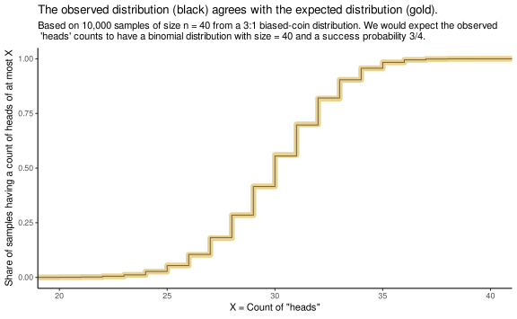
But maybe we just got lucky. As a stronger test of our SQL sampling logic, let’s take 10,000 samples of size 40 and look at the count of heads across all of the samples. We would expect this count to have a Binomial(size = 40, p = 3/4) distribution. To compare our observed results to the expected distribution, I’ll compute the empirical distribution of the results and plot that over the expected distribution. As you can see, the observed distribution closely matches the expected distribution:

When we take 10,000 independent samples of size n = 40 from a 3:1 biased-coin distribution, we find that the count of “heads” over the samples agrees with the expected Binomial(size = 40, p = 3/4) distribution.

Conclusion

Sampling is a powerful tool. And with the SQL logic we’ve just discussed, you can take fast, easy samples from virtually any dataset, no matter how large. And you can take those samples with or without replacement.

What makes it all work is a clever connection to the theory of Poisson processes. Those processes are memoryless and mergeable, and their arrivals win races in proportion to their rates. These properties are exactly what we need to run races that let us take samples.

Beyond what we’ve discussed in this article, there are further ways we can exploit these properties. For example, as a performance optimization, we can predict the arrival time t of the final row in a sample. Then we can augment our SQL sampling logic with a pushdown filter that eliminates population rows with arrival times greater than ct for some constant c. This filtering happens before ORDER/LIMIT processing and can greatly speed queries by eliminating more than 99.99% of rows early on, before they are even fully read on systems that support “late materialization.”

But this article is already too long, so I’ll stop here for now.

References

Pavlos S. Efraimidis and Paul G. Spirakis. Weighted random sampling with a reservoir. Information Processing Letters, 97(5):181–185, 2006.