Showing posts with label Statistics. Show all posts

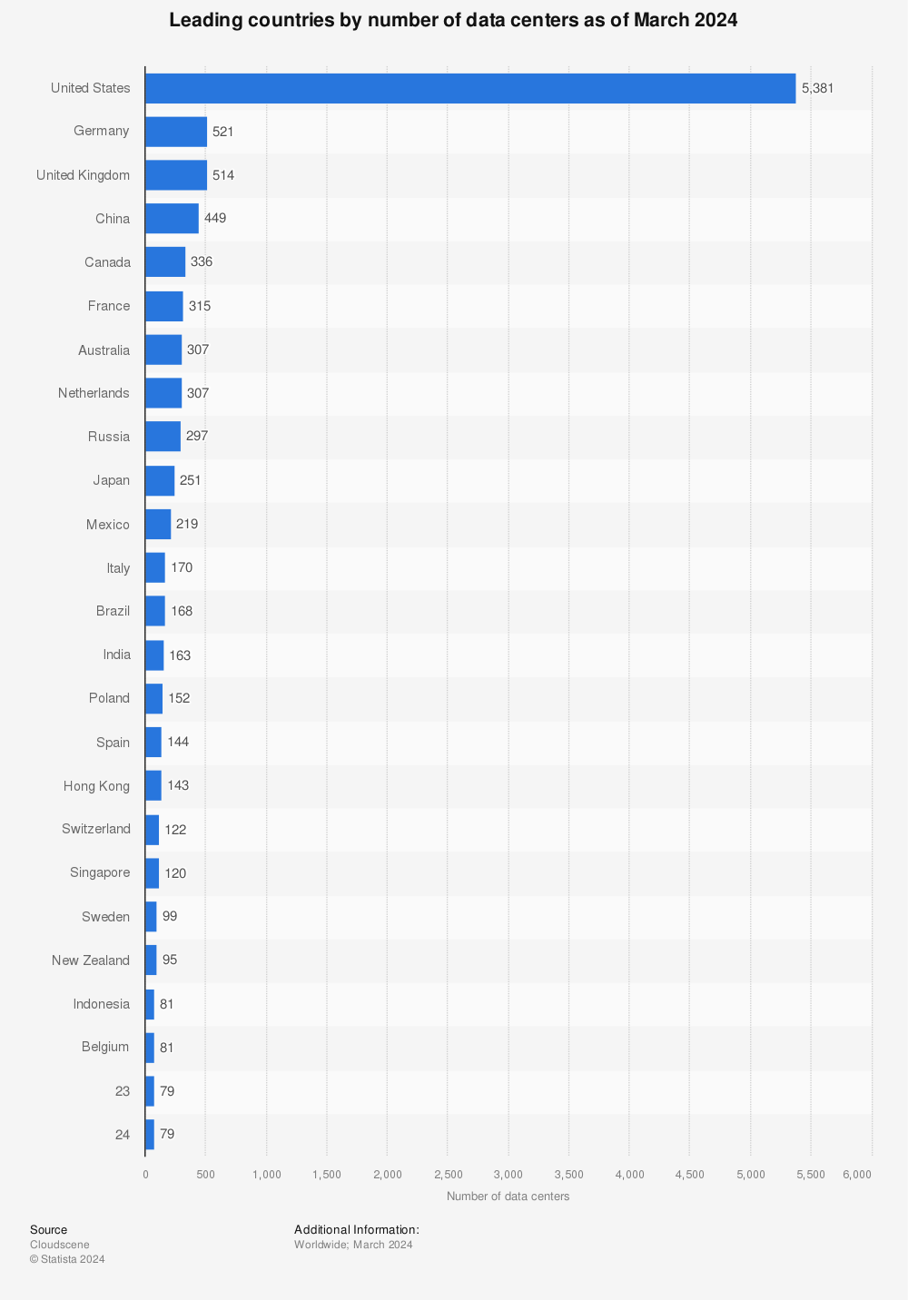
Number of data centers worldwide 2025, by country or territory

Mike's Notes

Provides some perspective on the distribution of their current locations. The 2025 data is available as a spreadsheet. 

It's also a proxy index of electrification and economic development by country.

Resources

References

  • Reference

Repository

  • Home > Ajabbi Research > Library >
  • Home > Handbook > 

Last Updated

25/12/2025

Number of data centers worldwide 2025, by country or territory

By: Petroc Taylor
Statistica: 19/11/2025

Petroc Taylor is a researcher with Statista's Technology and Telecommunications team. His research focus is global developments in the use of data, including trends in big data, analytics, and storage, as well as the impact of emerging data technologies across industries and sectors. He also supports the team's coverage of operating systems, telecommunications, and the technology industry in Africa..

As of November 2025, there were a reported 4,165 data centers in the United States, the most of any country worldwide. A further 499 were located in the United Kingdom, while 487 were located in Germany.

What is a data center?

Data centers are facilities designed to store and compute vast amounts of data efficiently and securely. Growing in importance amid the rise of cloud computing and artificial intelligence, data centers form the core infrastructure powering global digital transformation. Modern data centers consist of critical computing hardware such as servers, storage systems, and networking equipment organized into racks, alongside specialized secondary infrastructure providing power, cooling, and security.

AI data centers

Data centers are vital for artificial intelligence, with the world’s leading technology companies investing vast sums in new facilities across the globe. Purpose-built AI data centers provide the immense computing power required to train the most advanced AI models, as well as to process user requests in real time, a task known as inference. Increasing attention has therefore turned to the location of these powerful facilities, as governments grow more concerned with AI sovereignty. At the same time, rapid data center expansion has sparked a global debate over resource use, including land, energy, and water, as modern facilities begin to strain local infrastructure.

Data

Statistic: Number of data centers worldwide as of November 2025, by country or territory | Statista

Find more statistics at Statista

Bayesian Statistics

Mike's Notes

A great introduction to Bayesian Statistics. With example workbooks. All free, including an Excel Resource Pack. The Real Statistics website by Charles Zaiontz is a fantastic resource.

Update

The YouTube lesson by Vivek Vinushanth Christopher is superb.

Resources

References

  • Reference

Repository

  • Home > Ajabbi Research > Library >
  • Home > Handbook > 

Last Updated

24/01/2026

Bayesian Statistics

By: Charles Zaiontz
Real Statistics: 01/05/2021

Dr. Charles Zaiontz has a PhD in mathematics from Purdue University and has taught as an Assistant Professor at the University of South Florida as well as at Cattolica University (Milan and Piacenza) and St. Xavier College (Milan).

Bayesian statistics uses an approach whereby beliefs are updated based on data that has been collected. This can be an iterative process, whereby a prior belief is replaced by a posterior belief based on additional data, after which the posterior belief becomes a new prior belief to be refined based on even more data. The initial prior belief in this series may be based on intuition, previous studies, experience, etc.

In inferential statistics, we commonly test hypotheses, estimate parameters, and make predictions. In the traditional approach to statistics, commonly called the frequentist approach, parameters are constants whose values we aim to discern. Bayesian statistics uses a different approach: we treat these parameters as variables that have a probability distribution.

Topics

References

  1. Gelman, A., Carlin, J. B., Stern, H. S., Dunson, D. B., Vehtari, A., Rubin, D. B. (2014) Bayesian data analysis, 3rd Ed. CRC Press
    https://statisticalsupportandresearch.files.wordpress.com/2017/11/bayesian_data_analysis.pdf
  2. Marin, J-M and Robert, C. R.  (2014) Bayesian essentials with R. 2nd Ed. Springer
    https://www.springer.com/gp/book/9781461486862
  3. Jordan, M. (2010) Bayesian modeling and inference. Course notes
    https://people.eecs.berkeley.edu/~jordan/courses/260-spring10/lectures/index.html
  4. Lee, P. M. (2012) Bayesian statistics an introduction. 4th Ed. Wiley
    https://www.wiley.com/en-us/Bayesian+Statistics%3A+An+Introduction%2C+4th+Edition-p-9781118332573

Data Colada Table of Contents

Mike's Notes

Data Colada is a remarkable effort by Uri Simonsohn, Leif Nelson and Joe Simmons on topics such as fake data, research design, meta-analysis, and the reproducibility of science, among others.

Here is the table of contents of Data Colada.

Resources

References

  • Reference

Repository

  • Home > Ajabbi Research > Library >
  • Home > Handbook > 

Last Updated

26/09/2025

Data Colada Table of Contents

By: Uri Simonsohn, Leif Nelson and Joe Simmons.
Data Colada: 26/09/2025

Thinking about evidence and vice versa.


Table of Contents

About Research Design

About Research Tips

Comment on media coverage

Credibility Lab

Data Replicada

Discuss own paper

Discuss Paper by Others

Effect size

Fake data

file-drawer

Interactions

Just fun

Lawsuits

Meta Analysis

Music

On Bayesian Stats

Opinion

p-curve

p-hacking

Preregistration

Replication

Reproducibility

Researchbox

Statistical Power

Teaching

Unexpectedly Difficult Statistical Concepts

How to Learn the Math Needed for Machine Learning

Mike's Notes

An outline of what I need to study.

Resources

References

  • Reference

Repository

  • Home > Ajabbi Research > Library > Subscriptions > Towards Data Science
  • Home > Handbook > 

Last Updated

31/05/2025

How to Learn the Math Needed for Machine Learning

By: Edgor Howell
Towards Data Science: 15/05/2025

A breakdown of the three fundamental math fields required for machine learning: statistics, linear algebra, and calculus.

Maths can be a scary topic for people.

Many of you want to work in machine learning, but the maths skills needed may seem overwhelming.

I am here to tell you that it’s nowhere as intimidating as you may think and to give you a roadmap, resources, and advice on how to learn math effectively.

Let’s get into it!

Do you need maths for machine learning?

I often get asked:

Do you need to know maths to work in machine learning?

The short answer is generally yes, but the depth and extent of maths you need to know depends on the type of role you are going for.

A research-based role like:

  • Research Engineer — Engineer who runs experiments based on research ideas.
  • Research Scientist — A full-time researcher on cutting edge models.
  • Applied Research Scientist — Somewhere between research and industry.

You will particularly need strong maths skills.

It also depends on what company you work for. If you are a machine learning engineer or data scientist or any tech role at:

  • Deepmind
  • Microsoft AI
  • Meta Research
  • Google Research

You will also need strong maths skills because you are working in a research lab, akin to a university or college research lab.

In fact, most machine learning and AI research is done at large corporations rather than universities due to the financial costs of running models on massive data, which can be millions of pounds.

For these roles and positions I have mentioned, your maths skills will need to be a minimum of a bachelor’s degree in a subject such as math, physics, computer science, statistics, or engineering.

However, ideally, you will have a master’s or PhD in one of those subjects, as these degrees teach the research skills needed for these research-based roles or companies.

This may sound heartening to some of you, but this is just the truth from the statistics.

According to a notebook from the 2021 Kaggle Machine Learning & Data Science Survey, the research scientist role is highly popular among PhD and doctorates.

...

And in general, the higher your education the more money you will earn, which will correlate with maths knowledge.

...

However, if you want to work in the industry on production projects, the math skills needed are considerably less. Many people I know working as machine learning engineers and data scientists don’t have a “target” background.

This is because industry is not so “research” intensive. It’s often about determining the optimal business strategy or decision and then implementing that into a machine-learning model.

Sometimes, a simple decision engine is only required, and machine learning would be overkill.

High school maths knowledge is usually sufficient for these roles. Still, you may need to brush up on key areas, particularly for interviews or specific specialisms like reinforcement learning or time series, which are quite maths-intensive.

To be honest, the majority of roles are in industry, so the maths skills needed for most people will not be at the PhD or master’s level. 

But I would be lying if I said these qualifications do not give you an advantage.

What maths do you need to know?

There are three core areas you need to know:

  • Statistics
  • Calculus
  • Linear Algebra

Statistics

I may be slightly biased, but statistics is the most important area you should know and put the most effort into understanding.

Most machine learning originated from statistical learning theory, so learning statistics will mean you will inherently learn machine learning or its basics.

These are the areas you should study:

  • Descriptive Statistics — This is useful for general analysis and diagnosing your models. This is all about summarising and portraying your data in the best way.
    • Averages: Mean, Median, Mode
    • Spread: Standard Deviation, Variance, Covariance
    • Plots: Bar, Line, Pie, Histograms, Error Bars
  • Probability Distributions — This is the heart of statistics as it defines the shape of the probability of events. There are many, and I mean many, distributions, but you certainly don’t need to learn all of them.

    • Normal
    • Binomial
    • Gamma
    • Log-normal
    • Poisson
    • Geometric
  • Probability Theory — As I said earlier, machine learning is based on statistical learning, which comes from understanding how probability works. The most important concepts are

    • Maximum likelihood estimation
    • Central limit theorem
    • Bayesian statistics
  • Hypothesis Testing —Most real-world use cases of data and machine learning revolve around testing. You will test your models in production or carry out an A/B test for your customers; therefore, understanding how to run hypothesis tests is very important.

    • Significance Level
    • Z-Test
    • T-Test
    • Chi-Square Test
    • Sampling
  • Modelling & Inference —Models like linear regression, logistic regression, polynomial regression, and any regression algorithm originally came from statistics, not machine learning.

    • Linear Regression
    • Logistic Regression
    • Polynomial Regression
    • Model Residuals
    • Model Uncertainty
    • Generalised Linear Models

Calculus

Most machine learning algorithms learn from gradient descent in one way or another. And, gradient descent has its roots in calculus.

There are two main areas in calculus you should cover:

  • Differentiation
    • What is a derivative?
    • Derivatives of common functions.
    • Turning point, maxima, minima and saddle points.
    • Partial derivatives and multivariable calculus.
    • Chain and product rules.
    • Convex vs non-convex differentiable functions.
  • Integration

    • What is integration?
    • Integration by parts and substitution.
    • The integral of common functions.
    • Integration of areas and volumes.

Linear Algebra

Linear algebra is used everywhere in machine learning, and a lot in deep learning. Most models represent data and features as matrices and vectors.

  • Vectors 
    • What are vectors
    • Magnitude, direction
    • Dot product
    • Vector product
    • Vector operations (addition, subtraction, etc)
  • Matrices 
    • What is a matrix
    • Trace
    • Inverse
    • Transpose
    • Determinants
    • Dot product
    • Matrix decomposition
  • Eigenvalues & Eigenvectors 
    • Finding eigenvectors
    • Eigenvalue decomposition
    • Spectrum analysis

Best Resources

There are loads of resources, and it really comes down to your learning style.

If you are after textbooks, then you can’t go wrong with the following and is pretty much all you need:

  • Practical Statistics For Data Scientist — I recommend this book all the time and for good reason. This is the only textbook you realistically need to learn the statistics for Data Science and machine learning.
  • Mathematics for Machine Learning — As the name implies, this textbook will teach the maths for machine learning. A lot of the information in this book may be overkill, but your maths skills will be excellent if you study everything.

If you want some online courses, I have heard good things about the following ones.

  • Mathematics for Machine Learning and Data Science Specialisation — This course is by DeepLearning.AI, the same people who made the Machine Learning Specialisation, arguably the best machine learning course.

Learning Advice

The amount of maths content you need to learn may seem overwhelming, but don’t worry.

The main thing is to break it down step by step.

Pick one of the three: statistics, Linear Algebra or calculus.

Look at the things I wrote above you need to know and choose one resource. It doesn’t have to be any of the ones I recommended above.

That’s the initial work done. Don’t overcomplicate by looking for the “best resource” because such a thing doesn’t exist.

Now, start working through the resources, but don’t just blindly read or watch the videos.

Actively take notes and document your understanding. I personally write blog posts, which essentially employ the Feynman technique, as I am, in a way, “teaching” others what I know.

Writing blogs may be too much for some people, so just make sure you have good notes, either physically or digitally, that are in your own words and that you can reference later.

The learning process is generally quite simple, and there have been studies done on how to do it effectively. The general gist is:

  • Do a little bit every day
  • Review old concepts frequently (spaced repetition)
  • Document your learning
  • It’s all about the process; follow it, and you will learn!

Markov Blankets

Mike's Notes

Pipi uses Markov chains, which can form a Markov Blanket. Blankets can be aggregated and nested. The Royal Society paper "The Markov Blankets of Life: autonomy, Active Inference and the Free Energy Principle" is excellent.

A Markov blanket statistically defines a system's boundaries (e.g., a cell or a multicellular organism). It is a statistical partitioning of a system into internal and external states, and the blanket itself consists of the states that separate the two.

Resources

References

  • Reference

Repository

  • Home > Ajabbi Research > Library >
  • Home > Handbook > 

Last Updated

12/10/2025

A Markov Chain Theory of Self Organization

By: Jacob Calvert, Georgia Tech University 

YouTube: 14/11/2024


Fundamentals of statistical mechanics explain that systems in thermal equilibrium spend more time in states with greater order because these states have lesser energy. This explanation is remarkable, and powerful, because energy is a "local" property of states. Nonequilibrium systems, like living systems, can also exhibit order, but there is no property analogous to energy that generally explains why states with greater order tend to emerge. However, recent experiments suggest that a local property called rattling predicts which states are favored, at least for a broad class of nonequilibrium systems. In this seminar, I will present a simple theory of rattling that explains when and why it works, and I will demonstrate its application to systems across scientific domains. Surprisingly, the core idea of rattling is so general as to apply to equilibrium and nonequilibrium systems alike. (Joint work with Dana Randall.)

Markov Blanket

"In statistics and machine learning, when one wants to infer a random variable with a set of variables, usually a subset is enough, and other variables are useless. Such a subset that contains all the useful information is called a Markov blanket. If a Markov blanket is minimal, meaning that it cannot drop any variable without losing information, it is called a Markov boundary. Identifying a Markov blanket or a Markov boundary helps to extract useful features. The terms of Markov blanket and Markov boundary were coined by Judea Pearl in 1988. A Markov blanket can be constituted by a set of Markov chains." - Wikipedia.


Brandon Foltz on maths

Mike's Notes

I found this resource recently while looking for a good introduction to Markov Chains to share with someone.

Brendan Foltz has created an excellent set of free introductory resources on statistics, math, and other subjects. These are great for visual learners to grasp the main concepts.

The GitHub repository has lots of supporting materials.

Resources

References

  • Reference

Repository

  • Home > Ajabbi Research > Library >
  • Home > Handbook > 

Last Updated

17/05/2025

Article

By: Brendan Fotz
YouTube: 20/04/2025

My tutorials focus on Introductory Statistics, Finite Mathematics, Management Science, Operations Management and Basic Accounting. My videos are full-length lessons...so grab a drink and stick around! :) 

If you are on here trying to learn; you are my inspiration. I simply love to learn and I have an insatiable curiosity about the world. Education and sharing knowledge is my passion. While I need to support the channel financially, I am not trying to sell or promote anything but learning.  If you subscribe and click the bell icon, you will only get new video notifications.

Some of the problems I work come from textbooks I really like and I highly recommend taking a look at them.

Keep working hard, never stop learning, and thanks for watching!

"You must give some time to your fellow men. Even if it's a little thing, do something for others - something for which you get no pay but the privilege of doing it." - Albert Schweitzer

Statistical Laws in Complex Systems: Combining Mechanistic Models and Data Analysis by Eduardo G. Altmann

Mike's Notes

I discovered this fascinating book/paper by Eduardo G. Altmann listed in the weekly Complexity Digest.

"Provides an unifying approach to the study of statistical laws. It starts with simple examples and goes through more advanced time series and statistical methods. Presents the necessary material to analyze, test, and interpret results in existing and new datasets" - Complexity Digest

He is a Maths and Stats Professor in the Complex Systems and Data Science group at the School of Mathematics and Statistics at the University of Sydney, Australia.

Resources

References

  • Reference

Repository

  • Home > Ajabbi Research > Library >
  • Home > Handbook > 

Last Updated

17/05/2025

Statistical Laws in Complex Systems: Combining Mechanistic Models and Data Analysis

By: Eduardo G. Altmann

ArXiv: Submitted on 29/07/2024

Summary

Statistical laws describe regular patterns observed in diverse scientific domains, ranging from the magnitude of earthquakes (Gutenberg-Richter law) and metabolic rates in organisms (Kleiber's law), to the frequency distribution of words in texts (Zipf's and Herdan-Heaps' laws), and productivity metrics of cities (urban scaling laws). The origins of these laws, their empirical validity, and the insights they provide into underlying systems have been subjects of scientific inquiry for centuries. This monograph provides an unifying approach to the study of statistical laws, critically evaluating their role in the theoretical understanding of complex systems and the different data-analysis methods used to evaluate them. Through a historical review and a unified analysis, we uncover that the persistent controversies on the validity of statistical laws are predominantly rooted not in novel empirical findings but in the discordance among data-analysis techniques, mechanistic models, and the interpretations of statistical laws. Starting with simple examples and progressing to more advanced time-series and statistical methods, this monograph and its accompanying repository provide comprehensive material for researchers interested in analyzing data, testing and comparing different laws, and interpreting results in both existing and new datasets.

Read the 152 page pdf

Sampling with SQL

Mike's Notes

An excellent post by Tom Moertel on how to use SQL when sampling big datasets. The original article has better formatting.

Resources

References

  • Reference

Repository

  • Home > Ajabbi Research > Library >
  • Home > Handbook > 

Last Updated

18/05/2025

Sampling with SQL

By: Tom Moertel
Tom Moertel’s Blog: 23/08/2024

Tags: sampling, sql, probability, poisson process, exponential distribution, statistics

Sampling is one of the most powerful tools you can wield to extract meaning from large datasets. It lets you reduce a massive pile of data into a small yet representative dataset that’s fast and easy to use.

If you know how to take samples using SQL, the ubiquitous query language, you’ll be able to take samples anywhere. No dataset will be beyond your reach!

In this post, we’ll look at some clever algorithms for taking samples. These algorithms are fast and easily translated into SQL.

First, however, I’ll note that many database systems have some built-in support for taking samples. For example, some SQL dialects support a TABLESAMPLE clause. If your system has built-in support—and it does what you need—using it will usually be your best option.

Often, though, the built-in support is limited to simple cases. Let’s consider some realistic scenarios that are more challenging:

  • We want to be able to take samples with and without replacement.
  • We want to take weighted samples in which each item in the input dataset is selected with probability in proportion to its corresponding weight.
  • We want to support the full range of weights we might expect to see in a FAANG-sized dataset, say between 0 to 1020 for frequency distributions (e.g., clicks or impressions or RPC events) and between 0 to 1 with values as small as 1020 for normalized probability distributions. In other words, weights are non-negative numbers, possibly very large or very small.
  • We want to take deterministic samples. This property lets us take repeatable samples and, in some cases, helps query planners produce faster queries.

Sampling without replacement: the A-ES algorithm in SQL

In 2006, Pavlos S. Efraimidis and Paul G. Spirakis published a one-pass algorithm for drawing a weighted random sample, without replacement, from a population of weighted items. It’s quite simple:

Given a population V indexed by i=1n and having weights wi:

  1. For each vi in V, let ui=random(0,1) and ki=ui1/wi.
  2. Select the m items with the largest keys ki.

That algorithm has a straightforward implementation in SQL:

SELECT *
FROM Population
WHERE weight > 0
ORDER BY -LN(1.0 - RANDOM()) / weight
LIMIT 100  -- Sample size.

You’ll note that we changed the ordering logic a bit. A straight translation would have been

ORDER BY POW(RANDOM(), 1.0 / weight) DESC

Our translation

ORDER BY -LN(1.0 - RANDOM()) / weight

is more numerically stable and also helps to show the connection between the algorithm and the fascinating world of Poisson processes. This connection makes it easier to understand how the algorithm works. More on that in a moment.

Numerical stability and other tweaks

First, the numerical stability claim. Assume that our SQL system uses IEEE double-precision floating-point values under the hood. When the weights are large, say on the order of wi=1017, it doesn’t matter what the random value ui is. The corresponding sort key ki=ui1/wi will almost always be 1.0. Consider the interval 0.01ui1, representing 99% of the possible random values ui. This entire interval gets mapped to 1.0 when wi=1017:

# Python.
>>> w_i = 1e17
>>> math.pow(0.01, 1.0/w_i) == math.pow(1.0, 1.0/w_i) == 1.0
True

Likewise, when weights are small, say wi=1017, the corresponding sort key will almost always be zero. Consider the interval 0ui0.99, representing 99% of the possible random values ui:

>>> w_i = 1e-17
>>> math.pow(0.0, 1.0/w_i) == math.pow(0.99, 1.0/w_i) == 0.0
True

For very large (or small) weights, then, the straightforward implementation doesn’t work. The wanted sort ordering is destroyed when very large (or small) powers cause what should be distinct sort keys to collapse into indistinguishable fixed points.

Fortunately, logarithms are order-preserving transformations, so sorting by ln(ui1/wi)=ln(ui)/wi produces the same ordering as sorting by ui1/wi when we’re using mathematically pure real numbers. But the log-transformed version is much more stable when using floating-point numbers. Distinct random inputs ui now produce reliably distinct sort keys ki, even when the input weights wi are very large or very small:

>>> [math.log(u_i) / 1e17 for u_i in (0.01, 0.010001, 0.99, 0.990001)]
[-4.605170185988091e-17, -4.605070190987759e-17,
 -1.005033585350145e-19, -1.0049325753001471e-19]

>>> [math.log(u_i) / 1e-17 for u_i in (0.01, 0.010001, 0.99, 0.990001)]
[-4.605170185988091e+17, -4.605070190987758e+17,
 -1005033585350145.0, -1004932575300147.1]

As a final tweak, we negate the sort keys so that instead of sorting by ui1/wi descending, as in the original algorithm, we do an equivalent sort by ln(ui)/wi ascending. Note the leading minus sign. The rationale for flipping the sign will become apparent when we discuss Poisson processes in the next section.

One last numerical subtlety. Why do we generate random numbers with the expression 1.0 - RANDOM() instead of just RANDOM()? Since most implementations of RANDOM(), such as the PCG implementation used by DuckDB, return a floating-point value in the semi-closed range, they can theoretically return zero. And we don’t want to divide by zero. So we instead use 1.0 - RANDOM() to generate a random number in the semi-closed range, which excludes zero.

Does this algorithm actually work?

It’s not obvious that assigning a random number ui to every row i, then sorting rows on ln(ui)/wi, and finally taking the top m rows is a recipe that would result in a valid sample. But it does.

The clearest way to understand what’s going on is to first take a detour through the fascinating world of Poisson processes. In short, a Poisson process with rate λ is a sequence of arrivals such that the times between successive arrivals are all independent, exponentially distributed random variables with rate λ.

Poisson processes have some important (and useful!) properties:

  1. They are memoryless. No matter what has previously happened, the time until the next arrival from a Poisson process with rate λ is exponentially distributed with rate λ.
  2. They can be merged. If you have two Poisson processes with rates λ1 and λ2, the arrivals from both processes form a combined Poisson process with rate λ1+λ2. This holds for any number of processes.
  3. They win races in proportion to their rates. In a race between the very next arrival from a Poisson process with rate λ1 and the very next arrival from a Poisson process with rate λ2, the probability that the first process will win the race is λ1/(λ1+λ2).

Now that we know the basics of Poisson processes, there’s just one more tidbit we need:

  • The uniform–exponential bridge. If X is a random variable having a uniform distribution between zero and one, then ln(X)/λ has an exponential distribution with rate λ.

With the uniform–exponential bridge in mind, we can begin to see what the algorithm is doing when it assigns every row a key ki=ln(ui)/wi and sorts the population by that key. It’s running a race over all the rows in the population! In this race, each row arrives at the finish line at a time that’s an exponentially distributed random variable with a rate corresponding to the row’s weight wi. The first m arrivals form the sample.

To prove that this race does the sampling that we want, we will show that it is equivalent to a succession of one-row draws, each draw being fair with respect to the population that remains at the time of the draw. Let the population’s total weight be w, and consider an arbitrary row i with weight wi. The algorithm will assign it an exponentially distributed random variable with rate wi, which corresponds to the very next arrival from a Poisson process with the same rate.

Now consider all rows except i. They too correspond to Poisson processes with rates equal to their weights. And we can merge them into a combined process with rate jiwj=wwi.

Now, using the rule about Poisson races, we know that row i, represented by a process with rate λ1=wi, will win the race against those other rows, represented by a combined process with rate λ2=wwi, with probability

λ1λ1+λ2=wiwi+(wwi)=wiw.

And since we chose row i arbitrarily, the same argument applies to all rows. Thus every row’s probability of being drawn is equal to its weight in proportion to the population’s total weight. This proves that running a “race of exponentials” lets us perform one fair draw from a population.

But, after we’ve drawn one row, what’s left but a new, slightly smaller population? And can’t we run a new race on this slightly smaller population to correctly draw another row?

We can. And, since Poisson processes are memoryless, we do not have to generate new arrival times to run this new race. We can reuse the existing arrival times because the arrivals that have already happened have no effect on later arrivals. Thus the next row we draw using the leftover arrival times will be another fair draw.

We can repeat this argument to show that successive rows are chosen fairly in relation to the population that remains at the time of each draw. Thus algorithm A-ES selects a sample of size m by making m successive draws, each fair with respect to its remaining population. And that’s the proof.

Tricks for faster samples

Most large analytical datasets will be stored in a column-oriented storage format, such as Parquet. When reading from such datasets, you typically only have to pay for the columns you read. (By “pay”, I mean wait for the query engine to do its work, but if you’re running your query on some tech company’s cloud, you may actually pay in currency too.)

For example, if your dataset contains a table having 100 columns but you need only four of them, the query engine will usually only read those four columns. In row-oriented data stores, by contrast, you’ll generally have to decode entire rows, even if you only want four out of the 100 values in each row. Additionally, most column-oriented stores support some kind of filter pushdown, allowing the storage engine to skip rows when a filtering expression evaluates to false. These two properties—pay for what you read and filter pushdown—are ones we can exploit when taking samples.

Say we have a Population table with billions of rows and around 100 columns. How can we efficiently take a weighted sample of 1000 rows?

We could use the basic sampling formulation, as discussed earlier:

SELECT *
FROM Population
WHERE weight > 0
ORDER BY -LN(1.0 - RANDOM()) / weight
LIMIT 1000  -- Sample size.

But think about what the query engine must do to execute this query. It must read and decode all 100 columns for all of those billions of rows so that it may pass those rows into the sort/limit logic (typically implemented as a TOP_N operation) to determine which rows to keep for the sample. Even though the sample will keep only 0.00001% of those rows, you’ll have to pay to read the entire Population table!

A much faster approach is to only read the columns we need to determine which rows are in the sample. Say our table has a primary key pk that uniquely identifies each row. The following variant on our sampling formulation returns only the primary keys needed to identify the rows in the sample:

SELECT pk
FROM Population
WHERE weight > 0
ORDER BY -LN(1.0 - RANDOM()) / weight
LIMIT 1000  -- Sample size.

This variant only forces the query engine to read two columns: pk and weight: Yes, it still must read those two columns for the billions of rows in the table, but those columns contain small values and can be scanned quickly. After all, that’s what column-oriented stores are designed to do well. The point is that we’re not paying to read about 100 additional columns whose values we’re just going to throw away 99.99999% of the time.

One we have identified the rows in our sample, we can run a second query to pull in the full set of wanted columns for just those rows.

Adding determinism

Our sampling algorithm depends on randomization. If we run our algorithm twice with the same inputs, we’ll get different results each time. Often, that nondeterminism is exactly what we want.

But sometimes it isn’t. Sometimes, it’s useful to be able to control the dice rolls that the algorithm depends on. For example, sometimes it’s useful to be able to repeat a sample. Or almost repeat a sample.

To allow us to control the nature of the randomization used when we take samples, we must replace calls to RANDOM with a deterministic pseudorandom function. One common approach is to hash a primary key and then map the hashed value to a number in the range 

. The following DuckDB macro pseudorandom_uniform will do exactly that:

-- Returns a pseudorandom fp64 number in the range [0, 1). The number

-- is determined by the given `key`, `seed` string, and integer `index`.

CREATE MACRO pseudorandom_uniform(key, seed, index)

AS (

  (HASH(key || seed || index) >> 11) * POW(2.0, -53)

);

We can vary the seed and index parameters to generate independent random values for the same key. For example, if I fix the seed to “demo-seed-20240601” and generate random numbers for the key “key123” over the index values, I get 10 fresh random numbers:

SELECT

  pseudorandom_uniform('key123', 'demo-seed-20240601', i) AS u_key123

FROM RANGE(1, 11) AS t(i);

Ten random numbers for the key “key123” and seed “demo-seed-20240601”.

i u_key123

1 0.9592606495318252

2 0.6309411348395693

3 0.5673207749533353

4 0.11182926321927167

5 0.3375806483238627

6 0.12881607107157678

7 0.6993372364353198

8 0.94031652266991

9 0.17893798791559323

10 0.6903126337753016

To take deterministic samples, we just replace calls to RANDOM() with calls to our function pseudorandom_uniform().

Now that we can take deterministic samples, we can do even more useful things! For example, we can take samples with replacement.

Sampling with replacement

Earlier, we proved that the A-ES algorithm allows us to take a sample without replacement as a series of successive draws, each draw removing an item from the population, and each draw fair with respect to the population that remains at the time of the draw. But what if we wanted to take a sample with replacement? A sample with replacement requires us to return each item to the population as it is selected so that every selection is fair with respect to the original population, and individual items may be selected more than once.

Can we efficiently implement sampling with replacement in SQL? Yes! But it’s a little trickier. (I haven’t found this algorithm published anywhere; please let me know if you have. It took me some effort to create, but I wouldn’t be surprised if it’s already known.)

Think back to our correctness proof for the A-ES algorithm. For each row 

 having a weight, the algorithm imagined a corresponding Poisson process with rate and represented the row by the very next arrival from that process. That arrival would occur at time , where is a uniformly distributed random number in the range. Then the algorithm sorted all rows by their values and took the first arrivals as the sample.

With one minor tweak to this algorithm, we can take a sample with replacement. That tweak is to consider not just the very next arrival from each row’s Poisson process but all arrivals. Let denote the th arrival from row’s process. Since we know that in a Poisson process the times between successive arrivals are exponentially distributed random variables, we can take the running sum over interarrival times to give us the needed arrival times. That is,, where represents the th uniformly distributed random variable for row.

One minor problem with this tweaked algorithm is that a Poisson process generates a theoretically infinite series of arrivals. Creating an infinite series for each row and then sorting the arrivals from all of these series is intractable.

Fortunately, we can avoid this problem! Think about how the A-ES algorithm for taking a sample without replacement relates to our proposed intractable algorithm for taking a sample with replacement. We could describe the without algorithm in terms of the with algorithm like so: Prepare to take a sample with replacement, but then ignore all arrivals for; the remaining arrivals must be of the form, where indicates the corresponding row. Then take the first of these remaining arrivals as your sample, as before.

Now think about going the other way, from having a without-replacement sample and needing to construct a corresponding with-replacement sample. Let be the set of rows sampled without replacement. We know these rows were represented by a corresponding set of arrival times 

 for in. We also know that, had the sample been taken with replacement, the race would have included some additional arrival times for that could have displaced some of the winning rows in. But, crucially, we also know that if represents the set of rows in the corresponding sample with replacement, then must be contained within 

. This claim follows from the fact that if any arrival for does displace a row among the first arrivals, the requirement implies that the displacing row is a duplicate of some row 

 that arrived earlier in the sample at time; thus, displacement cannot introduce a new row from outside of.

Therefore, if we have a sample without replacement, we can construct a sample with replacement from its rows. We can ignore all other rows in the population. This makes the problem much more approachable.

So now we can see an algorithm taking shape for taking a sample with replacement of size:

First, take an -sized sample without replacement using the efficient A-ES algorithm.

For each sampled row in, generate arrivals for using the same pseudorandom universe that was used to generate.

Take the first  arrivals as the sample.

You may have noticed that step 2 of this algorithm requires us to create 

arrivals for each of the rows in. This step thus requires time. When is large, this time can be prohibitive.

Fortunately, we can use probability theory to reduce this cost to 

. The idea is that if row is expected to occur in the sample times, it is very unlikely to occur more than times. So we don’t need to generate a full arrivals for each row in ; we can get away with generating arrivals instead, for a suitably large to assuage our personal level of paranoia.

Here’s a sample implementation as a DuckDB macro:

-- Takes a weighted sample with replacement from a table.

--

-- Args:

--  population_table: The table to sample from. It must have a `pk` column

--    of unique primary keys and a `weight` column of non-negative weights.

--  seed: A string that determines the pseudorandom universe in which the

--    sample is taken. Samples taken with distinct seeds are independent.

--    If you wish to repeat a sample, reuse the sample's seed.

--  sample_size: The number of rows to include in the sample. This value

--    may be larger than the number of rows in the `population_table`.

--

-- Returns a sample of rows from the `population_table`.

CREATE MACRO sample_with_replacement(population_table, seed, sample_size)

AS TABLE (

  WITH

    -- First, take a sample *without* replacement of the wanted size.

    SampleWithoutReplacement AS (

      SELECT *

      FROM query_table(population_table::varchar)

      WHERE weight > 0

      ORDER BY -LN(pseudorandom_uniform(pk, seed, 1)) / weight

      LIMIT sample_size

    ),

    -- Compute the total weight over the sample.

    SampleWithoutReplacementTotals AS (

      SELECT SUM(weight) AS weight

      FROM SampleWithoutReplacement

    ),

    -- Generate a series of arrivals for each row in the sample.

    SampleWithReplacementArrivals AS (

      SELECT

        S.*,

        SUM(-LN(pseudorandom_uniform(pk, seed, trial_index)) / S.weight)

          OVER (PARTITION BY pk ORDER BY trial_index)

          AS rws_sort_key

      FROM SampleWithoutReplacement AS S

      CROSS JOIN SampleWithoutReplacementTotals AS T

      CROSS JOIN

        UNNEST(

          RANGE(1, CAST(2.0 * sample_size * S.weight / T.weight + 2 AS INT)))

        AS I(trial_index)

    )

  -- Form the sample *with* replacement from the first `sample_size` arrivals.

  SELECT * EXCLUDE (rws_sort_key)

  FROM SampleWithReplacementArrivals

  ORDER BY rws_sort_key

  LIMIT sample_size

);

Example of sampling with replacement

As an example of when we might want to sample with replacement instead of without, consider the following population table ThreeToOne that represents the possible outcomes of tossing a biased coin:


ThreeToOne population table.

pk weight

heads 3

tails 1

For this biased coin, “heads” is 3 times as likely as “tails.” We can simulate flipping this coin 10 times by sampling 10 rows from the ThreeToOne population table with replacement:

SELECT pk

FROM sample_with_replacement(ThreeToOne, 'test-seed-20240601', 10);

Results of drawing a 10-row sample with replacement from ThreeToOne.

pk

heads

heads

heads

tails

tails

heads

heads

heads

tails

heads

In this sample, we got 7 heads and 3 tails. On average, we would expect about 7.5 heads in each sample of size 10, so our observed sample is close to our expectations.

But maybe we just got lucky. As a stronger test of our SQL sampling logic, let’s take 10,000 samples of size 40 and look at the count of heads across all of the samples. We would expect this count to have a Binomial(size = 40, p = 3/4) distribution. To compare our observed results to the expected distribution, I’ll compute the empirical distribution of the results and plot that over the expected distribution. As you can see, the observed distribution closely matches the expected distribution:

When we take 10,000 independent samples of size n = 40 from a 3:1 biased-coin distribution, we find that the count of “heads” over the samples agrees with the expected Binomial(size = 40, p = 3/4) distribution.

Conclusion

Sampling is a powerful tool. And with the SQL logic we’ve just discussed, you can take fast, easy samples from virtually any dataset, no matter how large. And you can take those samples with or without replacement.

What makes it all work is a clever connection to the theory of Poisson processes. Those processes are memoryless and mergeable, and their arrivals win races in proportion to their rates. These properties are exactly what we need to run races that let us take samples.

Beyond what we’ve discussed in this article, there are further ways we can exploit these properties. For example, as a performance optimization, we can predict the arrival time t of the final row in a sample. Then we can augment our SQL sampling logic with a pushdown filter that eliminates population rows with arrival times greater than ct for some constant c. This filtering happens before ORDER/LIMIT processing and can greatly speed queries by eliminating more than 99.99% of rows early on, before they are even fully read on systems that support “late materialization.”

But this article is already too long, so I’ll stop here for now.

References

Pavlos S. Efraimidis and Paul G. Spirakis. Weighted random sampling with a reservoir. Information Processing Letters, 97(5):181–185, 2006.